Visualizing Newton's method using WebGL
An interactive renderer of Newton's method animations.
I made an effort to make this article readable on any browser, but it's much better with WebGL enabled, so I strongly recommend turning it on.
Knowing how this works is not required to enjoy the animations, so feel free to skip the math sections if they do not interest you (or if you already know all this).
WebGL did not work :(
It seems that WebGL didn't start. You can visit get.webgl.org to find out how to enable WebGL on your browser. You can also try another browser or maybe even your mobile phone. Or you can keep on reading — I've added some YouTube embeds and images for this case.
Newton's method video. Alternative link.
Newton's method
Newton's method is an algorithm for finding roots (also called zeroes) of a function — inputs for which the function becomes zero. In other words, solving
f(z) = 0
You might be familiar with finding the roots of the quadratic equation
az2 + bz + c = 0
using the quadratic formula
There are many functions that don't have analytic expressions like the one above for finding their roots. In these cases we can use a root-finding algorithm. Newton's method is such an algorithm for differentiable functions (which is most functions that you will normally encounter).
It starts with a guess z0 and then iterates the following expression until the values either converge or fail to converge.
where f′(z) is the derivative of f(z).
We will be working in complex numbers, which naturally lend themselves to 2D images. Compared to regular (real) numbers, complex numbers are pairs of numbers. A complex number z = x + y·i can be represented as a point on a 2D plane with coordinates x and y, or alternatively as a pair (x, y).
An example
Let's find the roots of f(z) = z3 + 1 with Newton's method — the general solution to cubic functions is a tad unwieldy. The derivative of f is f′(z) = 3z2. Our iteration becomes
z3 + 1
Starting with an arbitrarily picked z0 = 1, we get z1 = 1 − (13 + 1)/(3·12) = 1 − 2/3 = 1/3 = 0.333333…, then z2 = 1/3 − (1/27 + 1)/(3·1/9) = −25/9 = −2.777777…, and so on until the iteration converges at z8 = z9 = −1. And indeed, (−1)3 + 1 = 0.
From the fundamental theorem of algebra, we know that f(z) has exactly 3 complex roots, so we have two more to go. As shown in the table below, starting at 1i we get 0.5 + 0.866025i. The last root, 0.5 − 0.866025i can be found by starting at −i.
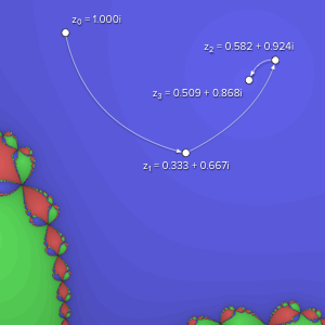
Iteration steps shown on the complex plane.
| Start at 1 | Start at 1i | |
|---|---|---|
| z0 | 1.000000 | 0.000000 + 1.000000i |
| z1 | 0.333333 | 0.333333 + 0.666667i |
| z2 | -2.77778 | 0.582222 + 0.924444i |
| z3 | -1.89505 | 0.508791 + 0.868166i |
| z4 | -1.35619 | 0.500069 + 0.865982i |
| z5 | -1.08536 | 0.500000 + 0.866025i |
| z6 | -1.00654 | 0.500000 + 0.866025i |
| z7 | -1.00004 | |
| z8 | -1.00000 | |
| z9 | -1.00000 |
Successive zn values.
Newton fractals
In our example, we saw that depending on the initial choice of z0, we can end up with different roots. The set of all initial values that give us a given root is called that root's basin of attraction.
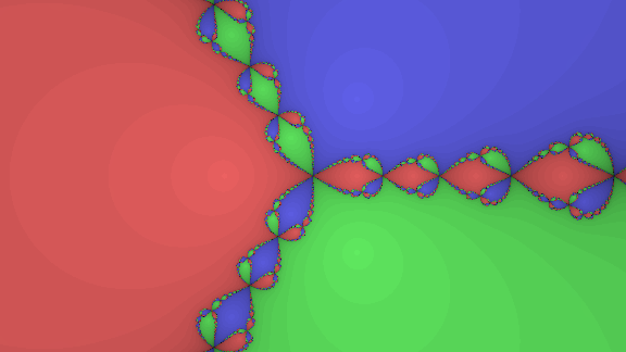
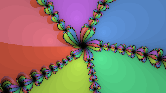
We can visualize Newton iteration by coloring every basin of attraction with a different color. For our equation, all the z0 values that end up at −1 will be red, the ones that give 0.5 + 0.866025i will be colored blue and the ones that give 0.5 − 0.866025i will be green.
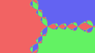
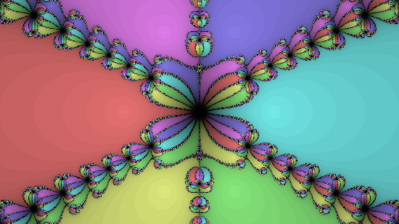
Basins of attraction for z3 + 1 colored red, blue and green (without shading).
We also saw that some guesses are better than others. z0 = 1 took 9 steps, while z0 = 1i was faster and only took 6 steps. We can use this to shade our image by the number of steps taken. Better initial guesses will be lighter and guesses that take a long time to converge will be dark.
This kind of visualization is called a Newton fractal.
Choosing pixel colors
An equation can have any number of roots. If we want to color each basin of attraction differently, we need to choose the colors algorithmically. This problem maps neatly onto the HSV color model. We choose a hue that corresponds to the root angle (the argument, or phase).
We set the color value (the V in HSV) based on the number of steps taken. This makes good starting points lighter and darkens those that converge slower.
One problem remains — what if two different roots have the same angle? That is, what if they lie on the same line starting at the origin? One such example is (z-1)·(z-2)·(z-3). To differentiate these, we set the saturation so that the closer the root is to 0, the more saturated it becomes.

(z-1)·(z-2)·(z-3)
float hue, saturation, v;

/* Choose a hue with the same angle as the argument */
hue = 0.5 + c_arg(z)/(PI*2.0);

/* Saturate roots the closer to 0 they are */
saturation = 0.59/(sqrt(c_abs(z)));

/* Make roots close to 0 white */
if (c_abs(z) < 0.1)
    saturation = 0.0;

/* Darken based on the number of steps taken */
v = 0.95 * max(1.0-float(steps)*0.025, 0.05);

/* Make roots with large values black */
if (c_abs(z) > 100.0)
    v = 0.0;
How this works
Generating these graphs is somewhat computationally intensive. Every pixel needs to perform a separate Newton iteration, the input functions can be complicated and they operate on complex numbers — pairs of floats, rather than floats themselves. Even something as simple as multiplication of two complex numbers takes a few operations.
complex c_mul(complex a, complex b)
{
    return complex(a.x*b.x-a.y*b.y, a.x*b.y+a.y*b.x);
}
Generating them in real-time, with a high resolution and frame rate in a high level language on the CPU is a nonstarter. Fortunately this problem lends itself really well to parallelization. And with today's powerful GPUs and increasing WebGL support, we can run the iteration in parallel in a browser. Breaking it down into steps, the process goes like this.
- Parse the equation into an abstract syntax tree
- Compute its derivative symbolically
- Generate the GLSL fragment shader
- Compile the shader and attach it to the WebGL context
- Run the shader for every pixel, every frame
Working with the equation
Newton's method requires us to compute the derivative of the function we want to solve. First we parse the equation into an abstract syntax tree (AST) using the nearley library.
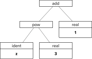
Abstract syntax tree for z3 + 1.
An AST will allow us to perform transformations on the equation, the first of which is to symbolically compute the derivative using differentiation rules.
| (f + g)′ = f′ + g′ | (c)′ = 0 |
| (f · g)′ = f′·g + f·g′ | (z)′ = 1 |
| (f / g)′ = (f′·g - f·g′)/g2 | (sin z)′ = cos z |
| (zn)′ = n·zn-1 | (cos z)′ = −sin z |
| (f(g))′ = f′(g)·g′ | (ez)′ = ez |
| (fg)′ = (eg·ln f)′ | (ln z)′ = 1/z |
Selected differentiation rules
Because the results of automatic differentiation can contain some unnecessary junk (such as multiplying a number by 1), we simplify the derivative AST by applying some common identities (such as 0 + z = z and 0 · z = 0) and we simplify some operations (replace 1 + 2 with 3). This helps with the frame rate, especially on slower machines. In our example, the differentiation yields 1·3·z3-1 + 0, which simplifies to just 3·z2.
Finally we convert the ASTs of both the original function and its derivative to GLSL, which is the C-based language shaders are written in. To put it simply, shaders are GPU programs. The bulk of our code is a fragment shader, which puts out a color for each pixel independently (and in parallel).
f = c_pow(z, complex(3.0, 0.0))) + (complex(1.0, 0.0))
df = c_mul(complex(3.0, 0.0), c_pow(z, complex(2.0, 0.0)))
Making it all interactive
We now have a way of rendering static Newton fractals relatively fast. We can take it a step further and animate it all. We'll introduce two parameters — real t for time and complex m for mouse coordinates. We declare the parameters as uniforms, which are shader input constants that stay the same across all pixels.
/* no typedef in GLSL so we use #define */
#define complex vec2

uniform complex m;
uniform complex t;
Every frame, we update the uniform values (without recompiling the shaders).
const m = gl.getUniformLocation(program, "m");
const t = gl.getUniformLocation(program, "t");

gl.uniform2f(m, mouseX, mouseY);
gl.uniform2f(t, time, 0.0);
Time
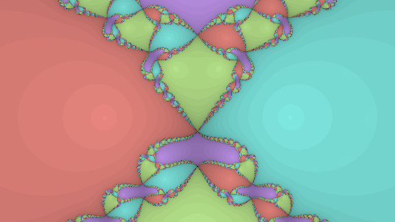
Using time as a real parameter allows us to look at how a fractal evolves as a term becomes dominant, for example the 4th degree term in z6 + 3·t·z4 - 10 or the constant term in z4 + 3·z2 + 2i·z - t - 1
z6 + 3·t·z4 - 10 at t = 0.5
z4 + 3·z2 + 2i·z - t - 1 at t = 30
We can also add an oscillation effect using sin(t), as in sin(z) + sin(t)·6i or a circular motion by exploiting cos(t) + i·sin(t) (or cis(t) for short), for example sec(z) + cis(t).
sin(z) + sin(t)·6i at t = 5.36
sec(z) + cis(t) at t = 10.7
Mouse position
Remember how complex numbers correspond to points on a plane? So do mouse positions! We set m to precisely the complex number pointed at by the cursor. This lets us get a better feel for the function, e.g. cos(z) + m. This works with touches on mobile devices too by the way.
We can use z2m + 1 to study how our earlier example z3 + 1 behaves as we change the exponent to fractional, negative and imaginary values.
z2m + 1 at m = 2.6 + 0.3i
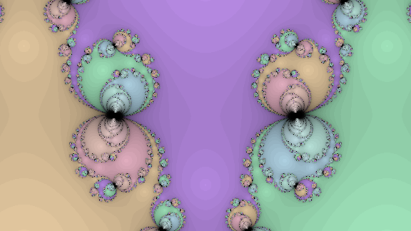
Another example is to add a root to a polynomial in factored form by multiplying it by (z-m), with m pointing at the new root: (z-1) · (z+2i) · (z-m).
(z-1) · (z+2i) · (z-m) at m = -3 + 0.9i
You can peek at the values for these parameters in real time by using the advanced tab.
Bonus for iPhones 6s and higher: touch force
Recent iPhones have a feature called 3D Touch, which measures how much force you're applying while touching the display, which I thought would be fun to add to the mix. We represent touch force by a real parameter f that runs from 0.0 to 1.0.
As an example, we can add it to our root factor's exponent in the previous example to play with the its order, like so: (z-1) · (z+2i) · (z-m)1+f.
canvasElement.addEventListener("touchforcechange", function(event) {
    if (event.touches.length !== 1) {
        /* Don't fire on multi-touch */
        return;
    }
    var touch = event.touches[0];

    setTouchForce(touch.force);

    event.preventDefault();
});

canvasElement.addEventListener("touchend", function(event) {
    setTouchForce(0.0);

    event.preventDefault();
});
Alternative algorithms
There are other root-finding algorithms that use derivatives. One of them is Halley's method. It converges faster than Newton's, but requires the computation (and the existence) of the second derivative (which is the derivative of the derivative). Fortunately once you can compute derivatives, you can compute second (and further) derivatives easily. However, for our purposes this method is usually slower because the second derivative tends to be much more complex.
Halley's method video. Alternative link.
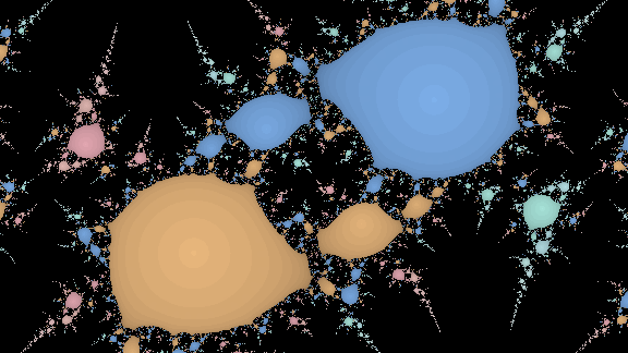
Another one of these is Householder's method, which also requires a second derivative. It's interesting to compare graphs generated with these to those generated with Newton's method — the differences as well as the similarities.
Householder's method.
A note on accuracy
Different WebGL implementations may produce slightly different results and sometimes glitches might show up. Also, there might be some bugs in the shader code, especially the more exotic complex functions — web GLSL isn't exactly easy to test.
Writing your own functions
You can write your own equations. One way to get started is by playing with existing functions — change the constants, add things, multiply by things, wrap things with functions, change functions to other functions, and so on. Let me know if you find anything interesting!
Available expressions
| Arithmetic | z+w, z-w, z*w, z/w, z^w |
| Trigonometric | sin(z), cos(z), tan(z), cot(z), sec(z), csc(z), cis(z) |
| Inverse trigonometric | asin(z), acos(z), atan(z), acot(z), asec(z), acsc(z) |
| Hyperbolic | sinh(z), cosh(z), tanh(z) |
| Other | sqrt(z), ln(z), exp(z), pi, e, i |
| Variables | m, t |
Tips
- To add a timed circular motion, use cis(t), which is short for cos(t) + i·sin(t).
- If you're getting a lot of black (divergence), add a simple term with z in it, or multiply the equation by z.
See also
Math
- The fast inverse square root algorithm, based on Newton's method, also known for the constant 0x5f3759df. It famously appeared in Quake III Arena.
- Fractals derived from Newton-Raphson iteration by Simon Tatham (you might know him as the author of PuTTY). He goes a bit more into the mathematics. He also describes a way of smoothing the fractals, but personally I kind of like them the way they are here.
- Newton's method at MathWorld.
WebGL
- Gregg Tavares' awesome WebGL Fundamentals.
- MDN WebGL docs.
- GLSL sandbox for playing around with shaders without any setup.
Code
- newton.js — this is what draws the fractals
- selectize.js — custom <select> control library
- nearley.js — parsing library